Regression analysis is a statistical method used to examine the relationship between two or more variables.
It helps us understand how the typical value of a dependent variable (the outcome we are interested in) changes when one or more independent variables (factors that might influence that outcome) are changed.
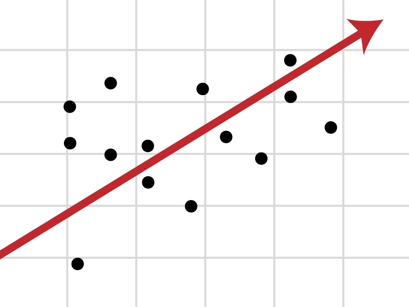
If x increases, does y also increase? or does y decrease? or does y stay the same?
The main purpose of regression analysis is to predict the value of a variable whose value we don’t know at the moment based on the values of known variables.
For example, we could use regression analysis to predict an athlete’s performance (which is unknown, as it’s in the future) based on their achievements in training to date (which we know).
Regression is a powerful tool for predicting and forecasting outcomes. By establishing the strength and nature of relationships between variables, regression analysis can help inform decisions about what matters. It tells us what might happen if we change something (for example, by increasing time in a certain area of training we’ll have x effect on performance).
In addition to prediction, regression analysis is crucial for understanding relationships between variables. This involves examining how variables are related and the nature of their relationship. For example, in environmental studies, researchers might use regression to understand how temperature affects plant growth. This analysis can provide insights into which factors are most important and how they interact with each other.
Important
Before moving on, it’s important to remind yourself about dependent and independent variables. In data analysis, the dependent variable is the outcome that we are interested in. It’s the ‘what will happen’ part of the question. Independent variables are things we suspect will influence that outcome.
The dependent variable is called DV and the independent variable IV.
It’s useful to think about independent variables as ‘predictors’, and dependent variables as ‘outcomes’. I’ve used this terminology at some points below. The outcome depends on the predictor.
7.2 Simple linear regression
Simple linear regression is a method used to model the linear relationship between two variables. In this context, we have one independent variable (predictor) and one dependent variable (response). As the name suggests, it’s the simplest form of regression.
What’s the difference between correlation and simple linear regression?
Correlation and simple linear regression are two statistical methods that seem similar because both deal with relationships between two variables, but they serve different purposes and provide different information.
Correlation: This is about measuring how strongly two variables are related to each other. For example, let’s say you’re looking at the amount of time spent studying and test scores. Correlation would tell you how closely these two things move together. If the correlation is high, it means that as study time goes up, test scores tend to go up too (and vice versa). But correlation doesn’t tell you anything about cause and effect; it just says these two variables are linked in some way. It’s often represented by a coefficient (like Pearson’s r), which ranges from -1 to 1, showing the strength and direction of the relationship.
Simple Linear Regression: This method takes it a step further. It not only looks at how two variables are related, but also tries to predict one variable based on the other. Using the same example, simple linear regression would help you predict test scores based on how much time a student spends studying. It gives you an equation (like y = mx + b, where ‘y’ is the predicted score, ‘m’ is the slope, ‘x’ is the study time, and ‘b’ is the y-intercept) that models this relationship. Regression can suggest cause-and-effect (though it doesn’t prove it) by showing how changes in one variable can lead to changes in another.
Basically, correlation measures the strength and direction of a relationship between two variables, while simple linear regression provides a way to predict the value of one variable based on the other.
The independent variable is used to predict the value of the dependent variable. For instance, we might use years of education (independent variable) to predict income (dependent variable).
Equation of a line
Simple linear regression is based on the assumption that the relationship between the two variables is linear.
What’s a linear relationship?
A linear relationship between two variables means that when one variable changes, the other changes at a constant rate.
Picture it like a straight line on a graph: one variable is on the horizontal axis (x-axis) and the other on the vertical axis (y-axis). As you move along the line, every step you take horizontally results in a consistent step vertically. This consistency is what makes the relationship ‘linear’.
It’s like walking up a ramp; the slope or steepness of the ramp stays the same.
Therefore, we try to create a line that best explains that relationship.
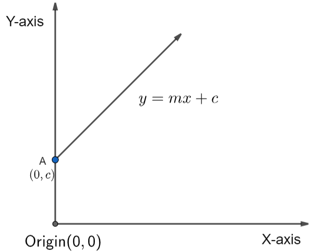
The ‘equation of a line’ in simple linear regression can be written as:
\[
y=mx+c
\] - y: This is the dependent variable (the outcome we are predicting)
x: The independent variable (the predictor)
m: Slope of the line (represents the change in y for a one-unit change in x)
c: y-intercept (value of y when x is 0)
This equation allows us to predict the value of y given a value of x.
Click here if you’re not following this!
Imagine you want to draw a straight line on a graph that shows the relationship between two things, like how far you throw and how many hours you train.
In linear regression, the “equation of a line” helps you draw this line.
The equation looks like this: y = mx + c. Here’s what each part means:
y: This is what you’re trying to predict or find out. For example, it could represent how far you will throw.
x: This is what you already know or can measure. It could be the number of hours you train
m: This is called the slope. It shows how much y changes when x changes. If the slope is big, it means doing a few more hours might increase your throw distance a lot. If the slope is small, even many more hours don’t add much to your distance.
c: This is the starting point of the line when x is zero, also known as the y-intercept. It’s like a throwing distance you’d achieve even if you did no training.
So, if you know how many training hours you’ve done (x), you can use this equation to estimate your throwing distance (y).
The line created by this equation on a graph would show you a trend or pattern of how your throwing changes with the number of hours training.
This helps in predicting and understanding how two things are related to each other. For example, you might discover that lots of hours training doesn’t actually add much value to your throwing distance!
Least squares method
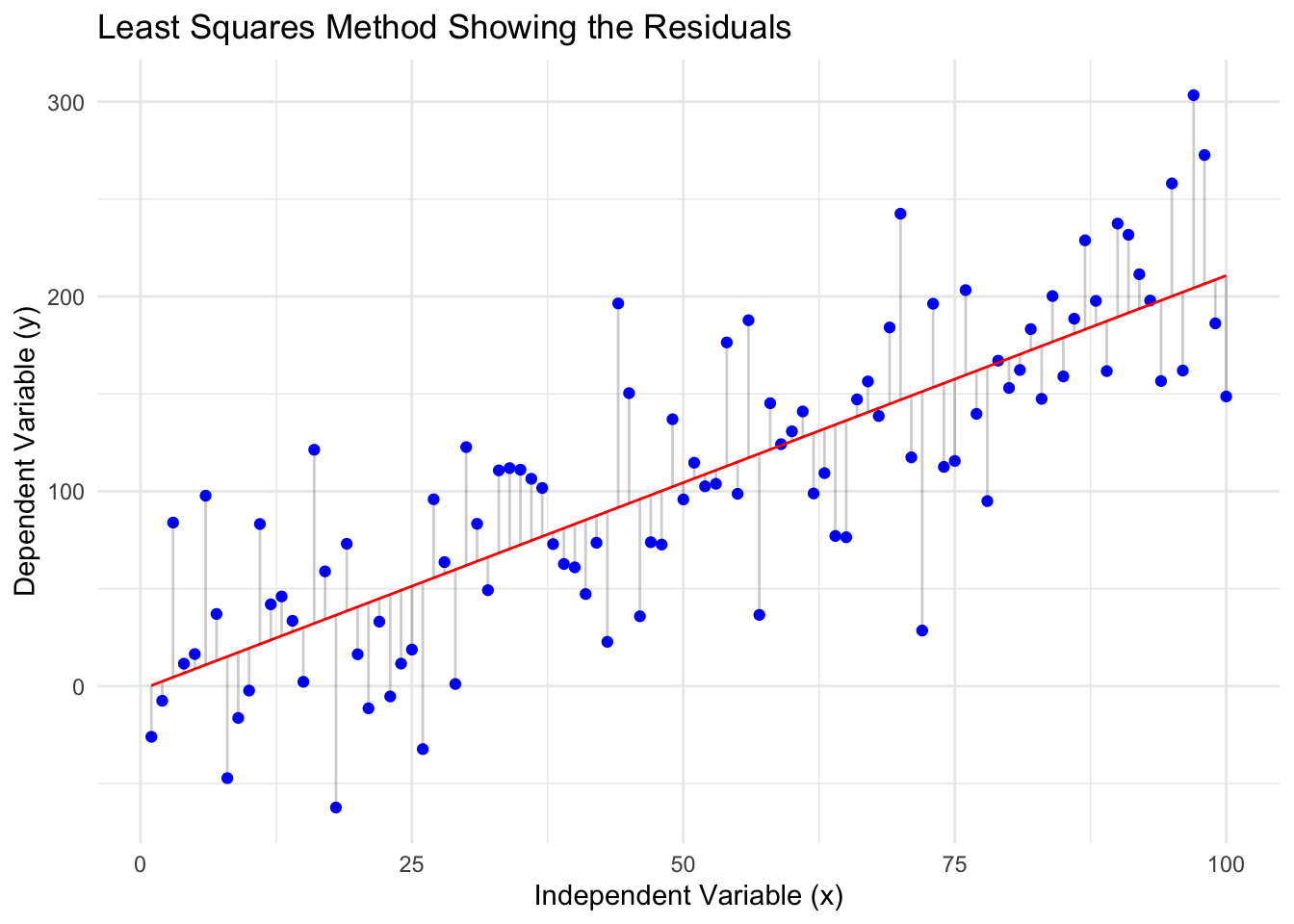
The ‘least squares’ method is used to find the best-fitting line through the data.
It does this by minimising the sum of the squares of the differences (residuals) between observed values and those predicted by the linear model. The ‘residuals’ are the distances from the actual data points to the line of best fit.
The following plot demonstrates this idea. The regression line (the line of best fit, in red) represents how the total distance between each value (in blue) has been reduced as far as possible, by producing as small residuals as possible.
Show code
# Load necessary librarieslibrary(ggplot2)# Generate synthetic dataset.seed(123) # For reproducibilityx <-1:100y <-2*x +rnorm(100, mean =0, sd =50) # Linear relationship with noise# Simple Linear Regression using Least Squares Methodmodel <-lm(y ~ x)# Predicted valuespredictions <-predict(model)# Residualsresiduals <- y - predictions# Data frame for ggplotdata <-data.frame(x, y, predictions, residuals)# Plottingggplot(data, aes(x, y)) +geom_point(aes(y = y), colour ="blue") +geom_line(aes(y = predictions), colour ="red") +geom_segment(aes(xend = x, yend = predictions), alpha =0.2) +labs(title ="Least Squares Method Showing the Residuals",x ="Independent Variable (x)",y ="Dependent Variable (y)") +theme_minimal()
Assumptions
All statistical tests are based on assumptions about the data that they are fed. It’s really important to know about these, as violating these assumptions can lead to completely unreliable analysis.
Simple linear regression is based on several key assumptions:
Linearity: The relationship between the independent and dependent variable should be linear. This means that we can assume that, as the independent variable increases, the dependent variable will also increase or decrease in a somewhat straight line.
Independence: Observations should be independent of each other.
Homoscedasticity: The variance of residual is the same for any value of the independent variable.
Normality: For any fixed value of the independent variable, the dependent variable should be normallydistributed.
More on homoscedasticity
Homoscedasticity is a fundamental assumption in regression analysis. It indicates that the variance of the errors (residuals) is consistent across all levels of the independent variables. This means that as the predictor variable changes, the spread or scatter of the residuals remains constant.
When homoscedasticity is present, it suggests that the model is well-specified and the error term behaves consistently across all values of the independent variables. This is important for the reliability of statistical tests and the creation of confidence intervals.
In contrast, heteroscedasticity, where the variance of residuals varies, can lead to inefficient estimates and affect the validity of hypothesis tests. Detecting homoscedasticity often involves visual methods like residual plots or statistical tests like the Breusch-Pagan test.
Example
Let’s use a simple example in R to illustrate simple linear regression. We’ll use the mtcars dataset, which is built into R.
First, we load the data (mtcars).
Then, we view the first 6 rows of the dataset (head).
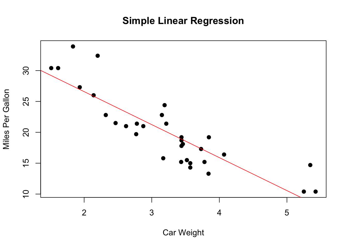
Then, we create a regression model which allows us to predict mpg using wt (weight).
We then ask for a summary of the model - this shows us that weight is a significant factor in predicting mpg.
The summary tells us that the direction of this association is negative - the estimate is -5.34 - so as weight gets higher, mpg gets lower.
We finish with a scatterplot of the two variables, and a linear regression line that provides a visual representation of the relationship.
# Load the datadata(mtcars)# View the first few rows of the datasethead(mtcars)
# Let's predict miles per gallon (mpg) using the weight of the car (wt)# Fit the linear modelmodel <-lm(mpg ~ wt, data = mtcars)# Summary of the modelsummary(model)
Call:
lm(formula = mpg ~ wt, data = mtcars)

Residuals:
    Min      1Q  Median      3Q     Max
-4.5432 -2.3647 -0.1252  1.4096  6.8727

Coefficients:
            Estimate Std. Error t value Pr(>|t|)
(Intercept)  37.2851     1.8776  19.858  < 2e-16 ***
wt           -5.3445     0.5591  -9.559 1.29e-10 ***
---
Signif. codes:  0 '***' 0.001 '**' 0.01 '*' 0.05 '.' 0.1 ' ' 1

Residual standard error: 3.046 on 30 degrees of freedom
Multiple R-squared:  0.7528,    Adjusted R-squared:  0.7446
F-statistic: 91.38 on 1 and 30 DF,  p-value: 1.294e-10
# Plottingplot(mtcars$wt, mtcars$mpg, main ="Simple Linear Regression", xlab ="Car Weight", ylab ="Miles Per Gallon", pch =19)abline(model, col ="red")
Reporting the results of a simple linear regression
A lot of this module will be concerned with learning about how to conduct various types of statistical analysis. However, we also need to know how to correctly report this analysis, for example within a professional report, dissertation, or scientific paper.
Key elements to include in such a report are:
Model Significance: Indicate if the overall model is statistically significant (using F-test and its p-value).
Regression Equation: Provide the estimated regression equation.
Coefficients: Report the coefficients (β values), including their significance (using t-tests and p-values).
Effect Interpretation: Describe how changes in the independent variable are associated with changes in the dependent variable.
Model Fit: Include the R² value to indicate how much variance in the dependent variable is explained by the model.
Statistical Significance: Always mention the p-values to discuss the significance of the findings.
So you might say something like:
“In our analysis, we conducted a simple linear regression to examine the relationship between car weight (independent variable) and miles per gallon (MPG, dependent variable) using the mtcars dataset. The results of the regression indicated that the model was statistically significant (F(1, 30) = 91.49, p < .001).
The regression equation for predicting MPG from car weight was: MPG = 37.29 - 5.34 × Car Weight. The coefficient for car weight was statistically significant (β = -5.34, t(30) = -9.56, p < .001), indicating that for each 1,000-pound increase in car weight, the MPG is expected to decrease by approximately 5.34 units.
The model explained a substantial proportion of variance in MPG, with an R² of .753. This means that approximately 75.3% of the variability in MPG can be explained by the car’s weight.
In conclusion, our analysis suggests a strong negative linear relationship between car weight and MPG, with heavier cars tending to have lower fuel efficiency.”
7.3 Multiple linear regression
Multiple linear regression extends simple linear regression by modeling the relationship between two or more independent variables and a single dependent variable.
It allows us to see how the dependent variable changes when multiple independent variables are varied.
This is particularly useful in ‘real-world’ scenarios in sport where the outcome is often influenced by more than one factor.
For example, predicting a team’s points total (dependent variable) based on previous goals scored, current points total, and number of shots on target (independent variables).
Equation of a line
In multiple linear regression, the equation is an extension of the simple linear model (Section 7.2.1):
\[
y = b0 + b1x1 + b2x2 +... +bnxn + ϵ
\] In this model:
y: Dependent variable
x1, x2,...,xn : Independent variables
b0 : y-intercept
b1, b2,...,bn : Coefficients of the independent variables
ϵ: Error term
Each coefficient represents the change in the dependent variable for a one-unit change in the corresponding independent variable, holding all other variables constant.
Remember, the only thing that is really changing here is that we are now including multiple IVs (predictors) into our model, rather than just one.
Least squares method
As for simple linear regression, the least squares method in multiple linear regression also aims to minimise the sum of the squares of the residuals.
However, it does this in a multidimensional space, as there are multiple independent variables.
Assumptions
As we noted previously, certain assumptions are made by statistical tests about your data. Assumptions of multiple linear regression (which you’ll note are very similar to those noted above for simple linear regression) include:
Linearity: The relationship between the independent variables and the dependent variable should be linear.
Independence: Observations should be independent of each other.
Homoscedasticity: The variance of the residuals should remain constant across all levels of the independent variables.
Normality: The residuals should be normallydistributed.
No Multicollinearity: The independent variables should not be too highly correlated with each other.
More on multicollinearity
Multicollinearity in statistical modeling, particularly in multiple linear regression, refers to a situation where two or more predictor variables are highly correlated with each other.
This high correlation means that these variables carry similar information about the variance in the dependent variable, making it challenging to isolate the individual effect of each predictor.
In the presence of multicollinearity, the statistical model becomes less reliable, particularly in terms of the interpretation of coefficients. Coefficients can become unstable and their estimates may change erratically in response to small changes in the model or data.
High multicollinearity can also inflate the standard errors of the coefficients, leading to a failure in identifying significant predictors even when they truly are.
It’s important to detect and address multicollinearity to ensure the validity and reliability of the regression analysis. Tools like the Variance Inflation Factor (VIF) can help quantify the level of multicollinearity and guide decisions on how to manage it, such as by removing or combining collinear variables.
Example
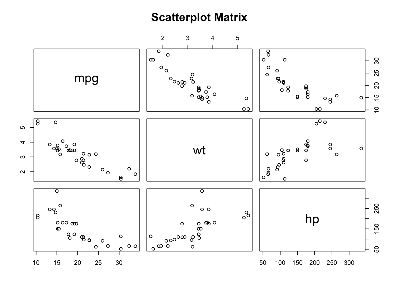
In the following example, we’ll examine the association between several predictors (wt and hp) on an outcome variable (mpg).
First, we load the dataset (mtcars).
Then, we create a model that includes both predictors (wt and hp).
We print a summary of our model. This tells us that both weight AND hp are significantly associated with mpg (weight at p < 0.001 and hp at p < 0.01). In both cases the estimate is negative, indicating that as each increases, mpg decreases.
Finally, we create a matrix of scatterplots that give a visual representation of these associations.
# Load the datadata(mtcars)# Fit the linear modelmodel <-lm(mpg ~ wt + hp, data = mtcars)# Summary of the modelsummary(model)
Call:
lm(formula = mpg ~ wt + hp, data = mtcars)

Residuals:
   Min     1Q Median     3Q    Max
-3.941 -1.600 -0.182  1.050  5.854

Coefficients:
            Estimate Std. Error t value Pr(>|t|)
(Intercept) 37.22727    1.59879  23.285  < 2e-16 ***
wt          -3.87783    0.63273  -6.129 1.12e-06 ***
hp          -0.03177    0.00903  -3.519  0.00145 **
---
Signif. codes:  0 '***' 0.001 '**' 0.01 '*' 0.05 '.' 0.1 ' ' 1

Residual standard error: 2.593 on 29 degrees of freedom
Multiple R-squared:  0.8268,    Adjusted R-squared:  0.8148
F-statistic: 69.21 on 2 and 29 DF,  p-value: 9.109e-12
# You can also use the 'pairs' function to create a matrix of scatterplots# to observe the relationships between variablespairs(~mpg + wt + hp, data = mtcars, main ="Scatterplot Matrix")
Reporting the results of a multiple regression analysis
Key elements of a report include:
Model Overview: Briefly describe the purpose of the model and the predictors used.
Statistical Significance of the Model: Report the F-statistic and its p-value.
Regression Equation: Provide the estimated regression equation.
Coefficients and Their Significance: Discuss the coefficients (β values) for each predictor, their t-statistics, and p-values.
Model Fit: Include R² and adjusted R² values.
Multicollinearity Assessment: Mention any tests used to assess multicollinearity.
Interpretation and Limitations: Offer insights based on the model’s findings and acknowledge its limitations, emphasizing the distinction between correlation and causation.
So you might use something like:
“Our analysis aimed to explore the determinants of fuel efficiency (measured in miles per gallon, MPG) in cars, using a multiple regression model with car weight (wt), horsepower (hp), and quarter-mile time (qsec) as predictors. The analysis was conducted using data from the mtcars dataset.
The multiple linear regression model was statistically significant (F(3, 28) = 26.62, p < .001), indicating that at least one of the predictors is significantly related to MPG. The regression equation was found to be: MPG = 30.68 - 3.92 × wt - 0.018 × hp + 0.865 × qsec.
In terms of individual predictors, car weight was negatively associated with MPG (β = -3.92, t = -4.67, p < .001), suggesting that heavier cars tend to have lower fuel efficiency. Horsepower was also negatively associated with MPG (β = -0.018, t = -2.08, p = .047), indicating a slight decrease in MPG with higher horsepower. Conversely, quarter-mile time was positively associated with MPG (β = 0.865, t = 2.91, p = .007), suggesting that cars with faster acceleration (lower qsec) tend to be less fuel-efficient.
The model accounted for approximately 84.4% of the variance in MPG (R² = .844), with an adjusted R² of 82.0%, indicating a strong fit with the data.
However, it is important to note that while the model shows significant associations, it does not imply causation.
In conclusion, the model suggests that car weight, horsepower, and quarter-mile time are significant predictors of fuel efficiency in the context of the mtcars dataset, with weight being the most influential factor.”
7.4 Interpretation of regression coefficients
When examining the output of regression models, it’s important to understand what the different outputs represent.
What is a ‘coefficient’?
In regression analysis, coefficients are values that represent the relationship between the independent variable(s) and the dependent variable.
Each coefficient indicates the expected change in the dependent variable for a one-unit change in the corresponding independent variable, holding all other variables constant.
For instance, in a regression model predicting house prices (dependent variable) from size (in square feet) and age (in years), the coefficient of size might indicate how much the price increases for each additional square foot, while the coefficient of age might show how much the price decreases for each year.
‘Standardised’ vs ‘unstandardised’ coefficients
These are shown as ‘Estimates’ in the R output above.
The choice between standardised and unstandardised coefficients depends on the context of the analysis.
Unstandardised coefficients (often simply called coefficients) are the raw coefficients obtained directly from the regression analysis. They are in the units of the dependent variable per unit of the independent variable. For example, in a model predicting weight gain (in kilograms) from calorie intake (in calories), an unstandardised coefficient of 0.002 would suggest a 0.002 kg increase in weight for each additional calorie consumed.
In contrast, standardised coefficients, also known as beta coefficients, are dimensionless and provide a way to compare the relative importance of different variables in the model. They are derived by standardising the variables before running the regression. A higher absolute value of a standardised coefficient implies a stronger influence of that variable on the dependent variable.
‘Significance’
The significance of regression coefficients is often determined using p-values and confidence intervals. A p-value is a measure of the probability that an observed effect could have occurred by random chance.
In general, a lower p-value (commonly below 0.05) suggests that the coefficient is significantly different from zero, indicating a meaningful contribution of the variable to the model.
Confidence intervals can provide a range within which we can be confident (usually 95%) that the true coefficient value lies. A confidence interval that does not include zero also indicates a significant effect.
Practical implications
Regression coefficients are not just numbers in a statistical output; they have practical implications. By understanding the magnitude and significance of these coefficients, decision-makers can make informed predictions and choices.
For example, in business, a company might use a regression model to decide where to allocate marketing resources, based on the coefficients indicating the effectiveness of different advertising channels. In healthcare, a model might help in understanding which clinical factors most significantly impact patient outcomes, guiding treatment approaches.
7.5 Reading
For further reading on regression, I’d recommend you take a look at the following book, which is available via the University library through the module reading list on myplace:
Fahrmeir, L. (2021). Regression : models, methods and applications / [internet resource] (T. Kneib, S. (Stefan M. ) Lang, & B. D. Marx, Eds.; Second edition..). SPRINGER.